
Testing How LLM Inference Scales Across GPUs
I was testing Llama 3.1 8B on A100 GPUs, and I expected the results to be easy to explain: four GPUs should be faster than two, which should be faster than one. The plots mostly showed that, but I still did not know what had actually improved. Was it the time before the first token, the time between generated tokens, or just less time waiting in a queue?
To answer that, I went back to vLLM's benchmark output, server logs, and an NVIDIA Nsight trace of the four-GPU run. The rest of this post follows the questions that came out of that: how a prompt becomes tokens, where the GPU time goes, and why more GPUs sometimes help.
Experiment at a glance
- Model and topology
- Llama 3.1 8B on 1, 2, or 4 NVIDIA A100-SXM4-40GB GPUs
- Server
- vLLM 0.10.1rc2.dev263+g2f13319f4 · bfloat16
- Load
- 200 prompts at 12 requests/s
- Prompt distribution
- 12–16,000 tokens; median 1,601, mean 1,506; two 16K-token prompts
- Output distribution
- 2–1,585 tokens; median 343, mean 393
- Fixed server flags
- --swap-space 16 --enforce-eager --enable-chunked-prefill --max-num-batched-tokens 512 --max-num-seqs 64 --disable-sliding-window
- What changed
- Only tensor-parallel size, and therefore the 1-, 2-, or 4-GPU allocation, across TP1, TP2, and TP4
Baseline results
| Configuration | p50 TTFT | p99 TTFT | p50 TPOT | p99 TPOT | Req/s · tok/s |
|---|---|---|---|---|---|
| TP1 · 1 GPU | 4,964 ms | 21,169 ms | 32.81 ms | 41.38 ms | 3.88 · 1,524 |
| TP2 · 2 GPUs | 2,732 ms | 12,139 ms | 23.39 ms | 28.64 ms | 4.78 · 1,877 |
| TP4 · 4 GPUs | 2,208 ms | 7,726 ms | 19.96 ms | 22.31 ms | 5.34 · 2,097 |
TTFT and TPOT are in milliseconds. Throughput is completed requests per second and generated output tokens per second.
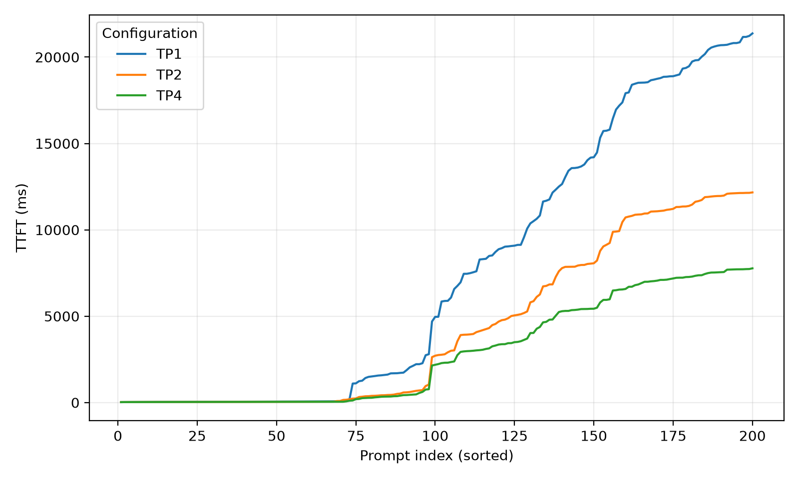
The first TTFT plot was the clue. Across most of this workload, the four-GPU configuration sits below the one- and two-GPU configurations. That only becomes useful after separating the two phases of generation.
The Dichotomy of LLM Inference
When you send a prompt to a generative model, it does not immediately begin the familiar one-token-at-a-time loop. First it runs prefill: it processes every token already in the prompt and builds the attention state it needs. Only then does decode begin, where it generates the response token by token.
Inside each transformer layer, the prompt is projected into queries, keys, and values. A query asks which earlier tokens matter; it is compared with keys, and the resulting attention weights select from values. Prefill does this for the full prompt and stores its keys and values in the KV cache. During decode, the new token creates one more query, key, and value, then attends over that cached history. Keeping the cache is what avoids recomputing the entire prompt for every new token, but the cache still has to be read and grows with the context.
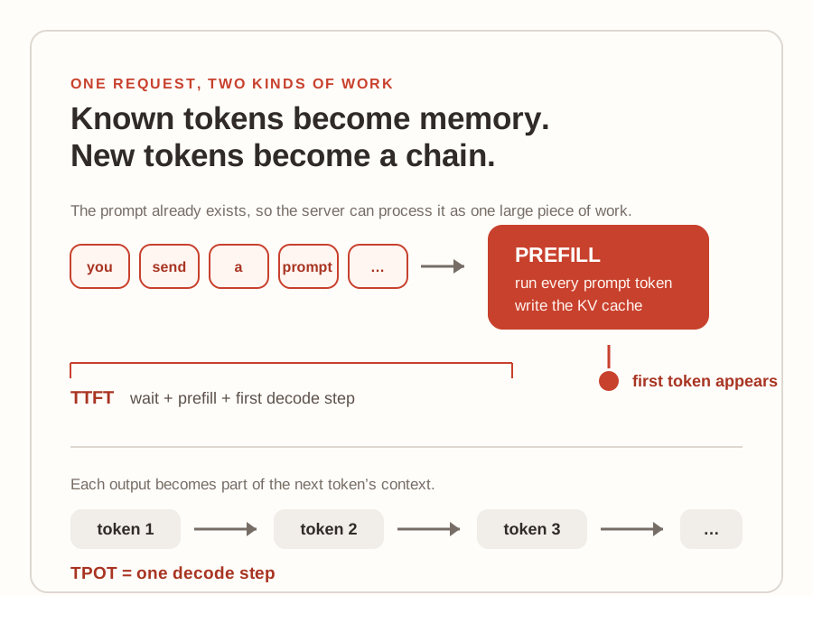
During prefill, the prompt already exists, so vLLM can batch its work through every layer and write attention keys and values into the KV cache, the request's working memory. Longer prompts mean more work before anything appears. Decode is different: token 12 cannot exist until token 11 does. The server can batch many requests, but it cannot generate one request's future tokens in parallel. This gives two useful measurements: TTFT for getting to the first token and TPOT for the rhythm after that.
A roofline view on an A100
Roofline modeling gave me a useful way to reason about this without treating GPU utilization as one number. It plots arithmetic intensity, operations per byte moved, against achieved FLOP/s. At low arithmetic intensity, performance follows the memory-bandwidth ceiling: moving bytes is the limit. At high arithmetic intensity, it reaches the flat compute ceiling: the math units are the limit. The crossover is the roofline's ridge point.
AI = FLOPs / bytes movedP ≤ min(P_peak, AI × BW_peak)AI* = P_peak / BW_peak ≈ 200 FLOP/byte on an A100The 40 GB A100s used here have about 1.555 TB/s of HBM bandwidth and up to 312 TFLOP/s of FP16/BF16 Tensor Core throughput. As a rough peak-based calculation, that puts the ridge point near 200 FLOP/byte. It is a useful scale, not a measurement of an actual kernel: precision, kernel shape, cache hits, and Tensor Core utilization all change what is achievable.
For Llama 3.1 8B, prefill is usually closer to compute-bound. Processing many prompt positions turns the linear layers into large matrix-matrix multiplies, so the same weights are reused across many tokens and the Tensor Cores have enough work to stay busy. Decode at low concurrency is usually closer to memory-bound. It generates only one new token per request, so it repeatedly streams model weights and reads the KV cache while doing relatively little math per byte. Attention itself is mixed: long-context prefill has substantial attention compute, while long-context decode increasingly pays for reading the cache. These are tendencies, not labels to apply blindly to every kernel; layer norms, cache writes, softmax, and communication have their own limits.
Metrics We Use
- TTFT: time to first token. The delay between sending a request and receiving its first generated token; it includes queueing, scheduling, and prompt processing.
- TPOT: time per output token. The average delay between later generated tokens; it is the streaming speed after the answer has started.
- p50 and p99. p50 describes a typical request. p99 exposes the slowest one percent of requests, the tail users are more likely to notice.
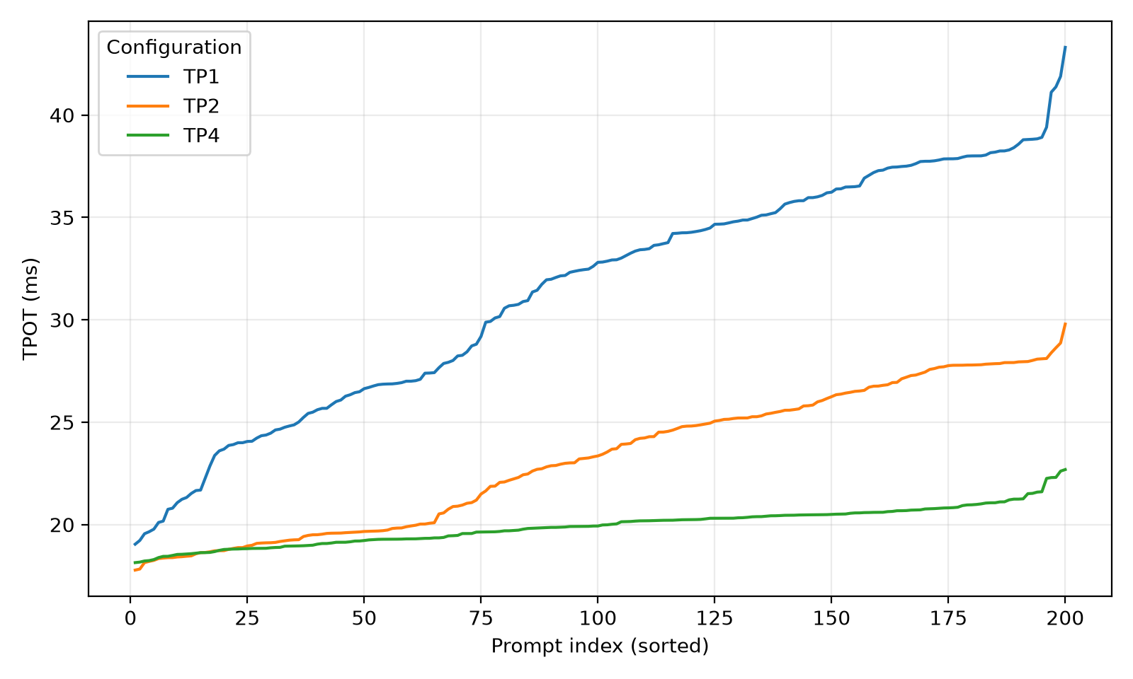
The TPOT curves show that tensor parallelism substantially reduced the time between generated tokens as work scaled from one to four GPUs, even with the added cross-GPU communication cost. The TPOT tail shows residual decode variability.
vLLM
vLLM is the serving layer between a client and the GPUs. It accepts API requests, tokenizes them, schedules prefill and decode work into GPU batches, manages KV-cache memory, and streams generated tokens back. Its scheduler decides whether a request can run now or must wait. max-num-seqs is a whole-engine concurrency cap: when it is full, new requests queue. Raising it can reduce that queueing, but it also makes more requests compete for GPU time and KV cache, which can worsen TPOT.
GPU Scaling Strategies
Tensor parallelism
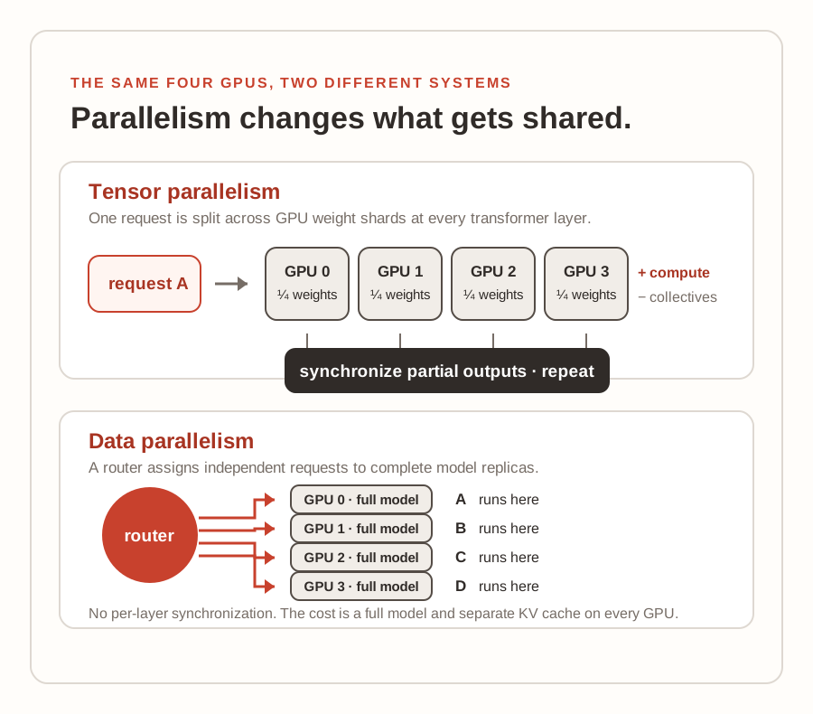
With tensor parallelism, one model execution is split across GPUs. TP4 means all four GPUs cooperate on the same request. Each GPU does part of the large tensor operations, then the partial results have to be combined before the next layer can continue. That can make one request faster, but it creates communication work on the critical path.
TP4 is one four-person team working on every layer. Each GPU multiplies a weight-matrix shard, then the partial outputs are assembled or summed with collectives such as AllReduce. Those collectives synchronize the GPUs, so a fast GPU can still wait for the slowest. The tradeoff is added cross-GPU communication and synchronization cost. TP makes sense when the matrix work it saves is larger than that cost, or when the model simply does not fit on one GPU.
Why tensor parallelism affects TPOT and TTFT differently
This helped me understand why TP often helps TPOT. Decode is a serial chain, so making one decode step shorter is the direct way to stream one request faster. TP can also speed prefill, but TTFT includes queueing, admission, and CPU/network overhead that TP cannot remove.
The roofline view explains part of that result. For memory-bound decode, tensor parallelism shards the weights, so each GPU reads only part of them and the request can use more aggregate memory bandwidth. The cost is that every layer now needs collective communication. For compute-heavy prefill, TP can split the large matrix multiplies too, but batching already gives an A100 a lot of useful work. Whether TP helps more than it communicates is still an experiment, not an assumption.
Data parallelism, or model replicas
Data parallelism creates four TP1 replicas, each with a full model and independent KV cache. A router sends one request to one replica. Under load, this is strong for TTFT because several requests can begin prefill instead of queueing behind one engine. It does not make an admitted request's TP1 prefill or decode faster, so it only improves TPOT indirectly when it prevents contention.
Data-parallel tradeoffs
The benefit is higher aggregate capacity and smaller independent queues. The cost is that every GPU stores a full model and its own KV cache, so replicas use more total memory and do not accelerate a single request the way tensor parallelism can. Routing also matters: a simple load balancer can distribute requests evenly, but it may not account for a replica with a long queue or a warm prefix cache.
Who actually routes a request?
Outside vLLM's built-in data-parallel mode, replicas need a router in front of them. NGINX, Envoy, HAProxy, Kubernetes, and Ray Serve solve variations of that problem. A simple router distributes HTTP requests; a better one can use queue length, cache pressure, or prefix affinity because every replica has its own queue and KV cache.
Tensor parallelism gives one request a team of GPUs. Data parallelism gives many requests separate copies of the model. The load balancer decides which copy receives each request.
Profiling: where are the GPUs actually spending time?
The benchmark showed what changed; NVIDIA Nsight helped explain it. The TP4 GPU kernel summary showed vLLM's custom cross-device reduction as the largest kernel, accounting for 59.2% of kernel time in this trace.
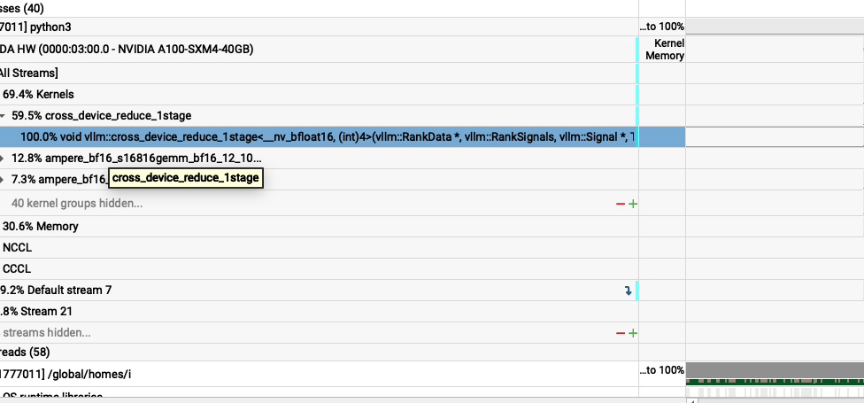
That reduction is the communication side of tensor parallelism: GPUs compute pieces independently, then need to combine them. Seeing 59.2% there did not mean TP4 was automatically wrong. My end-to-end measurements still gave TP4 the best TTFT and TPOT in this workload. The profile explained a cost inside the system; it did not replace the user-visible measurements.
Other knobs I would reach for

These are some of the knobs I played with to understand inference and workloads better. Each one moves one bottleneck and creates another tradeoff, so the useful approach is to name the symptom first, then change one variable.
- max-num-seqs: reduce queueing; watch TPOT and KV-cache pressure.
- max-num-batched-tokens and chunked prefill: balance GPU utilization against decode fairness.
- gpu-memory-utilization and max-model-len: trade safety margin for KV-cache capacity and context length.
- Prefix caching: reuse prefill only when prefixes genuinely repeat.
- tensor-parallel-size and data-parallel-size: choose whether GPUs cooperate on one request or serve independent ones.
enforce-eager is for debugging or profiling, not a free speed knob. Keep workload settings fixed, change one server setting, and compare TTFT, TPOT, throughput, cache use, and profiler evidence together.
A small experiment: was queueing the real bottleneck?
At 12 QPS, TP4 completed 5.34 requests/s under the 64-sequence cap, so I tested whether admission pressure was contributing to tail TTFT. I changed only that setting, increasing max-num-seqs from 64 to 128, and reran the same TP4 workload.
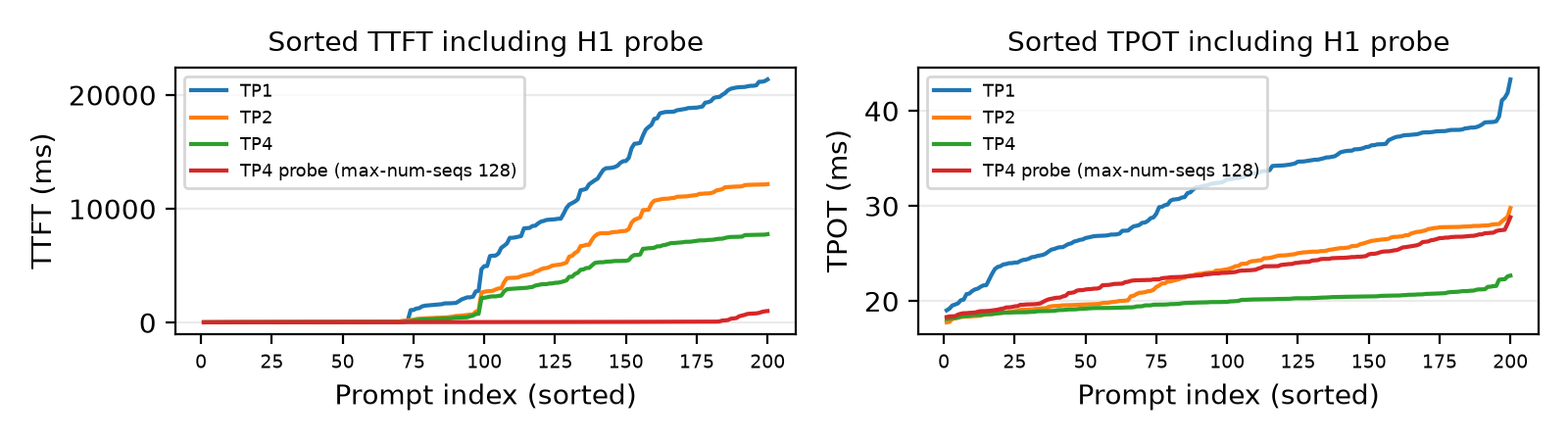
The result made the metric split concrete. p99 TTFT dropped from 7,726 ms to 938 ms, an 87.9% reduction. Median TPOT rose from 19.96 ms to 23.01 ms, a 15.3% increase. More active sequences meant less waiting before the first token, while the extra concurrent work made each decode step a little more expensive.
That does not make 128 universally correct; it supports admission pressure as a contributor to tail TTFT for this workload.
What I Learned
The main thing I learned is that I did not really understand how tensor parallelism worked before running this. Llama 3.1 8B can fit on one A100, so I initially thought data-parallel replicas might be the obvious way to use more GPUs. Replicas do split independent requests, but they do not split one request's layer-by-layer work.
The tradeoff is more specific than “more GPUs are faster.” Tensor parallelism can lower a single request's TPOT by sharding its compute and weight traffic, but it adds collective communication at every layer. Data parallelism improves aggregate capacity and queueing-driven TTFT because several requests can start on separate replicas, but it does not inherently make one request's decode faster. Prefill is usually closer to compute-bound; low-concurrency decode is usually closer to memory-bound. Those distinctions made the GPU results easier to reason about.
- Start with TTFT, TPOT, throughput, and tail latency; then use logs and profilers to identify which bottleneck to test next.
- Change one knob at a time and keep results, logs, profiler output, and scripts reproducible.